Evelyne Groen
Discussion: uncertainty and sensitivity analysis in environmental modelling
1. Background
The challenge to produce food in an environmentally friendly way has become urgent [Steinfeld et al., 2006; Gerber et al., 2013]. To develop strategies to produce food with a low environmental impact, environmental assessment models are developed that quantify the total environmental impact associated with food production, such as life cycle assessment or nutrient balance analysis. Input data required for these environmental impact assessment models, however, may vary due to seasonal changes, geographical conditions or socio-economic factors (natural variability) Moreover, input data may be uncertain, due to measurement errors and observational errors that exist around modeling of emissions and technical parameters (epistemic uncertainty). Although agricultural activities and food production are prone to natural variability and epistemic uncertainty, very few case studies made a thorough examination of the effects of variability and uncertainty on the result.
The aim of this thesis was to enhance understanding the effects of variability and uncertainty on the results. This was done by exploring how uncertainty analysis and sensitivity analysis can help to reduce the efforts for data collection, support the development of mitigation strategies and improve overall reliability, leading to more informed decision-making in environmental impact assessment models. To that end, methods for uncertainty analysis and sensitivity analysis were combined, and the effect of correlations in uncertainty propagation and global sensitivity analysis were explicitly accounted for. To be able to formulate case study specific suggestions that could improve reliability and point to potential mitigation strategies in food production, methods were applied to case studies of dairy and pork production.
This section starts with discussing the value of uncertainty analysis and sensitivity analysis in environmental impact assessment models, followed by the value of matrix notation. Subsequently, recommendation of the use of methods for uncertainty and sensitivity analysis are given. This section ends with an overview of the conclusions.
2. The value of uncertainty analysis and sensitivity analysis in environmental impact assessment models
2.1 Local sensitivity analysis
Local sensitivity analysis in environmental impact assessment models, such as life cycle assessment (LCA) and nutrient balance (NB) analysis, are generally performed using a one-at-a-time (OAT) approach. An OAT approach takes a parameter, increases it e.g. 5% and quantifies the effect on the model output. OAT approaches in LCA or NB analysis usually consider a subset of all available parameters, based on expert judgment or perhaps a quantitative criterion, such as the contribution of the individual input parameter to the total environmental impact. However, when the selection of the input parameters considered for the local sensitivity analysis is based on such principles, influential (technical) parameters might be overlooked. For example, efficiency parameters (e.g. replacement rate or reproductive performance) are not directly related to emissions, only to their prior production processes. These subsets, therefore, might not contain all potential influential parameters. A systematic approach that considers the influence of all input parameters in LCA can only be done using the multiplier method.
For example, in [Wolf and Groen et al., 2016], the multiplier method was used to identify the most influential parameters in an LCA that assessed greenhouse gas (GHG) emissions of milk production. Results showed that local sensitivity analysis identified milk yield, feed intake, and the emission factor of CH4 from enteric fermentation of the cows, replacement rate and crop yields as most influential parameters in the LCA model. Moreover, previous studies performing a local sensitivity analysis using an OAT approach, overlooked influential parameters such as replacement rate and crop yields.
In contrast to LCA, no such a systematic method is yet available for matrix-based NB analysis, Currently, studies that did performed a local sensitivity analysis, performed followed an OAT approach [Suh and Yee, 2011]. Future research can focus on developing a similar approach for matrix-based NB analysis.
Some LCA and NB studies [Huang et al., 2013; Kim and Dale, 2002; Sayagh et al., 2010; Beltran et al., 2016], use a sensitivity analysis to refer to the effect of different modeling decisions on the model output, such as the effect of changing allocation techniques or characterization factors. An explanation might be that ISO 14044 [2006] recommends performing a sensitivity analysis, which is defined as “systematic procedures for estimating the effects of the choices made regarding methods and data on the outcome of a study” [ISO 14044, 2006]. This definition not only refers to data, but also to methods used in a study, which indeed could refer to different allocation methods and characterization factors. Although the effect of a methodological decision, such as the allocation method used, is very important to the model outcome and the subsequent interpretation, they should not be referred to as sensitivity analysis. Moreover, the ISO standard does not make a distinction between a local sensitivity analysis (which does not include information of the uncertainty or variability around input parameters) and a global sensitivity analysis (which does include uncertainty or variability). The lack of distinction between local and global sensitivity analysis, has led in some studies [Flysjö et al., 2011; Basset-Mens et al., 2005] to include information about the uncertainty of the input parameters in, what is referred to as, a sensitivity analysis.
For example, Basset-Mens et al. [2005] explored the effect of an increase of 1% for some parameters, that were assumed to vary only little, and 200% for other parameters, that were assumed to vary a lot. Results in Groen et al. [2016], for example, showed that influential parameters in an LCA study of pork production were the feed conversion ratio, CH4 emissions from manure management and crop yields, especially maize. However, previous studies on this topic [Basset-Mens et al., 2005; Basset-Mens and van der Werf, 2005] included uncertainty ranges of the input parameters as well, and could therefore not comparable with the results presented in Groen et al. [2016].
Referring to modeling decisions as a sensitivity analysis or including uncertainty information in a OAT approach leads to an ambiguous definition of the terminology of uncertainty and sensitivity analysis, because:
- referring to a change in method or modeling structure has nothing to do with the intrinsic sensitivity of the model, and should therefore be given a different label, such as modeling decisions;
- combining uncertainty information in an OAT approach belongs to the area of screening analysis, which is strictly speaking not a local sensitivity analysis [Saltelli et al., 2008; Mutel et al., 2013];
- if uncertainty information is included in an OAT approach, it becomes less evident what it means to mutually compare the parameters, because it does not give the influence of the input parameters to the model output, as the magnitude of the uncertainty is incorporated as well.
Developing a standardized definition and method for local sensitivity analysis in LCA and NB analysis, will increase comprehensibility between studies and will enhance comparability of results.
2.2 Uncertainty analysis
Uncertainty propagation refers to propagation of uncertainty and variability around input parameters through an environmental impact assessment model to generate output data. Uncertainty analysis refers the subsequent analysis of the generated output data, such as determining the output variance, determining a confidence interval etc. Uncertainty propagation can be done using e.g. sampling approaches or analytical approaches.
For example, in [Groen et al., 2014], three sampling approaches (i.e. Monte Carlo sampling, Latin hypercube sampling, quasi Monte Carlo sampling), one analytical approach (i.e. on the basis of a Taylor series), and one fuzzy approach (i.e. fuzzy interval arithmetic) were compared, based on convergence rate and output statistics. The sampling methods led to more (directly) usable information, compared to fuzzy interval arithmetic or analytical uncertainty propagation. Latin hypercube and quasi Monte Carlo sampling provided more accuracy in determining the sample mean than Monte Carlo sampling. The Latin hypercube and quasi Monte Carlo sampling methods also converged faster than Monte Carlo sampling for some of the case studies discussed in [Groen et al., 2014]. The application of the more advanced sampling methods, therefore, might be less fruitful for applications in LCA, as the improvement mainly manifested itself in the number of runs generated. This seems less relevant in environmental impact assessment models, because the algorithm behind LCA and NB analysis does not require much run time. The latter depends on the specific software used and the capacity of the computer, nonetheless, classical Monte Carlo sampling seems a valuable sampling method to apply in LCA and NB studies.
The preference of a sampling approach versus an analytical for uncertainty propagation can depend on the amount of available information. A sampling approach requires a distribution function, including a parameter of dispersion such as the variance. Analytical uncertainty propagation as described in [Groen et al., 2014], does not require a distribution function, but only a parameter of dispersion. When less data is available about the uncertainty or variability of the input parameters, the analytical approach will become more suitable.
In [paper under review], for example, we used an NB to benchmark nutrient losses on farms for two different farming systems. Our aim was to explore the impact of measurement errors (epistemic uncertainty) on the benchmarking of farms within two different farming systems. The first farming system contained intensive farms, in terms of e.g. milk production per hectare (ha) and purchased concentrates per cow, whereas the second system included grass-based farms, with a lower milk production per ha. The distribution function and the parameters of dispersions of parameters required to assess the NB were obtained from the literature. We assumed that the epistemic uncertainties around the nitrogen flows were measured at different locations, using different measurement tools, and, therefore, could vary independently from each other. Uncertainty propagation could be performed using Monte Carlo sampling. The uncertainty analysis showed that benchmarking of concentrate-based farms was no longer possible when the epistemic uncertainty of input parameters was included, whereas including epistemic uncertainty did not affect benchmarking of grass-based farms.
In [Wolf and Groen et al., 2016], where we assessed greenhouse gas (GHG) emissions of milk production, a correlation was assumed between N-fertilizer application and crop yield; and between feed intake and milk production. Again, uncertainty propagation was performed using a sampling approach. We showed that, in the uncertainty analysis, the correlation between feed intake and milk production decreased the output variance.
To implement a correlation coefficient between input parameters during uncertainty propagation, as done in Wolf and Groen et al., [2016], information is needed not only on the distribution functions, but also on the correlation coefficients between input parameters. Using a sampling approach for uncertainty propagation with correlated input parameters, therefore, becomes even more data intensive. In Groen and Heijungs [2016] , therefore, we demonstrated how to predict the effect of ignoring correlations in uncertainty analysis in LCA, using analytical uncertainty propagation. More detailed, in Groen and Heijungs [2016] we demonstrated that:
- we can predict if including correlations among input parameters in uncertainty propagation will increase or decrease output variance;
- we can quantify the risk of ignoring correlations on the output variance and the global sensitivity indices.
This procedure requires only little data availability regarding the input parameters.
We conclude, therefore, that both sampling and analytical uncertainty propagation are indispensible in environmental impact assessment models. The analytical approach is especially useful when data is limited (e.g. only the variance of the input parameters is available). In contrast, the sampling approaches are more suitable when full knowledge is available (e.g. a distribution function, including a parameter of dispersion).
2.3 Global sensitivity analysis
A global sensitivity analysis quantifies the contribution of the variances of the individual input parameters to output variance. More specifically, a sensitivity index explains how much each input parameter contributes to the output variance. For example, the squared standardized regression coefficients can be interpreted as a sensitivity index.
For example, in [paper under review], we compared rather common methods for global sensitivity analysis in LCA, namely methods based on regression or correlation approaches [Geisler et al., 2005] and key issue analysis [Heijungs, 1996], to less commonly applied methods in LCA, such as the Sobol’ method and random balance design. The comparison of the sensitivity methods was based on four aspects: (I) sampling design, (II) output variance, (III) explained variance, and (IV) contribution to output variance of individual input parameters, and illustrated for two hypothetical case studies. The evaluation of the sampling design (I) relates to the computational effort of a sensitivity method. Key issue analysis does not make use of sampling (it is an analytical approach) and was fastest, whereas the Sobol’ method had to generate two sampling matrices, and therefore, was slowest. The total output variance (II) resulted in approximately the same output variance for each method, except for key issue analysis, which underestimated the variance, especially for high input uncertainties. The explained variance (III) and contribution to variance (IV) for small input uncertainties, was optimally quantified by standardized regression coefficients and the main Sobol’ index. For large input uncertainties, Spearman correlation coefficients and the Sobol’ indices performed best. Therefore, it was concluded that these less commonly applied methods did not outperform the common methods. Moreover, they asked for more unconventional algorithms, and may be more cumbersome to implement compared to the more frequently used methods based on linear regression or correlation approaches. However, the use of the Sobol’ method seemed better at explaining the output variance when input uncertainties are high. Also, other studies showed that the Sobol’ method might be more useful in the impact assessment model [Cucurachi et al., 2014]. Also, when the impact on the environment is quantified such as for toxicity, which contains potential non-linear relations [Posthuma et al., 2002] the Sobol’ method might become more useful.
If future environmental impact assessment studies become more advanced in terms of including non-linear impact assessment, the Sobol’ and random balance design methods as discussed in [paper under review], may become more useful. Based on the results presented in [paper under review], the squared standardized regressions coefficient (or the squared correlation coefficient), is considered as the most useful proxy for a global sensitivity index.
For example, in [paper under review], where we used an NB to benchmark nutrient losses on farms for two different farming systems, a global sensitivity analysis was applied using the squared standardized regression coefficients. We found that parameters that explained most of the output variance differed between systems. For the more concentrate-based system, input of feed and output of roughage were most important, whereas for the grass-based system, the input of mineral fertilizer (or fixation) was most important. Moreover, we showed that reducing epistemic uncertainty of the most important input parameters significantly improved benchmarking results.
In Wolf and Groen et al., [2016] we identified the most important input parameters to assess the greenhouse gas emissions of milk production, for three different grazing systems. We adapted the regression-based global sensitivity analysis to allow for correlated input parameters between feed intake and milk yield; and fertilizer rate and crop yield. We showed that the emissions factor of CH4 emission from enteric fermentation of cows, milk yield, feed intake and the emission factor of direct N2O emissions from crop cultivation, are the most important parameters for a zero grazing system. For restricted and unrestricted grazing systems, however, N2O emission factor from manure excretion during grazing becomes increasingly more important. When comparing the results of other studies to our results, we found that e.g. Ross et al. [2014] calculated the regression coefficients, so we could only compare their results based on the ranking of the parameters, and not on how much the parameters explained.
Several studies implemented regression coefficients (not standardized and not squared) [Basset-Mens et al., 2009; Aktas and Bilec, 2012], or standardized regression coefficients (not squared) [Sugiyama et al., 2005; Vigne et al., 2012], or correlation coefficients (not squared) [Mattila et al., 2012; Mattinen et al., 2014; Wang and Shen, 2013] as a measure for a global sensitivity index. For example, regression or correlation coefficients that are not squared, for example, cannot be mutually compared, and are therefore less suitable as a measure for a global sensitivity index. In Table 1, based on the case study represented in [paper under review], the squared standardized regression coefficients and the squared (Pearson) correlation coefficients were compared to the standardized regression coefficients, the regression coefficients and the correlation coefficient.
Table 1: Comparison of the regression and correlation coefficients, applied to the case study presented in [paper under review] (in adapted form) containing six input parameters. In the last row, the total explained output variance is given. Only the squared standardized regression and squared correlation coefficients can be added up, and are expressed in (%), the other coefficients cannot be added up, displayed by not applicable (n.a.) in the last row. CV: coefficient of variation (σ/μ); RC: regression coefficients; CC: correlation coefficients.| Parameter (CV) | Analysis of output variance by: | ||||
|---|---|---|---|---|---|
| Squared standardized RC | Standardized RC | RC | Squared CC | CC | |
| 1. (15.0%) | 58.1% | -0.762 | -13.0 | 56.4% | -0.751 |
| 2. (11.5%) | 1.08% | -0.104 | -11.6 | 1.15% | -0.107 |
| 3. (-) | - | - | - | - | - |
| 4. (20.0%) | 3.53% | -0.188 | -0.241 | 5.10% | -0.226 |
| 5. (15.0%) | 34.7% | 0.589 | 100 | 35.9% | 0.599 |
| 6. (8.00%) | 0.45% | 0.0699 | 2.13 | 0.590% | 0.0766 |
| Sum: | 99.0% | n.a. | n.a. | 99.0% | n.a. |
For example, ranking the importance of the parameters in Table 1, in case of the (squared) standardized regression coefficients or the (squared) correlation parameter 1 is most important, but when looking at the regression coefficients, parameter 5 is most important. The squared standardized regression coefficient or the squared correlation coefficient are the most useful proxies for a global sensitivity index, because they can be added to each other.
Currently in the ISO standard for LCA, there is no method recommended for a global sensitivity analysis. Developing a standardized definition and method for global sensitivity analysis in LCA and NB studies, will increase comprehensibility between studies and will enhance the comparison of results between studies.
2.4 The value of matrix notation in environmental impact assessment models
The environmental impact assessment models described in this thesis, LCA and NB analysis, both rely on matrix notation, to facilitate the application of uncertainty and sensitivity analysis. In matrix notation, the production processes are described by technical parameters given in the A-matrix. The corresponding emissions (and resource use) is given in the B-matrix. One may wonder, does matrix notation have any added value for sensitivity analysis? Uncertainty propagation using Monte Carlo simulation and global sensitivity analysis by means of standardized regression coefficients can also be performed for environmental impact models that do not make use of matrix notation. However, performing an analytical local sensitivity analysis that considers all input parameters, such as the multiplier method, applied in Groen et al. [2016] and Wolf and Groen et al., [2016], requires a functional form of the impact assessment model, such as the matrix-based approach developed by [Heijungs and Suh, 2002]. Although other functional forms have been proposed [Ciroth et al., 2004; Clavreul et al., 2013], in this context, matrix notation seems to be the most straightforward approach.
When we also consider correlations between input parameters, the algebraic notation gives clear insight into the effect of the correlations on the uncertainty propagation [Groen and Heijungs, 2016] . Using matrix notation, it was possible to predict the effect of including correlations during uncertainty propagation on the output variance and the global sensitivity analysis. Without the matrix formulation, it would have been impossible to make a sweeping generalization towards all different kind of case studies. To facilitate sensitivity analysis, matrix notation in LCA may not be eminent to implement uncertainty and sensitivity analysis, but is facilitates the algorithm implementation required to perform the methods, which otherwise would have been cumbersome to implement.
In Groen et al. [2016] and Wolf and Groen et al., [2016], greenhouse gas emissions were calculated for pork production and milk production respectively. To quantify the greenhouse gasses for crop cultivation, manure management and enteric fermentation, equations were implemented between the technical parameters in the A-matrix (e.g. fertilizer applied, manure produced and feed intake) and the GHG emissions in the B-matrix. For example, for the emissions of crop cultivation, the CO2 and indirect and direct N2O emissions depended directly on the application of fertilizers and crop yield.
The aggregation level of the production process determined which parameters showed up in the local and global sensitivity analysis.
For example, in Groen et al. [2016], we showed that CH4 emissions of manure turned out to be influential. However, the sensitivity analysis was modeled on the level of the total emissions, reflecting the parameters in the A- and B-matrix. Therefore, the influence of underlying factors determined by the type of manure storage system, such as the methane producing capacity, depending on temperature, wind speed etc., remains unknown.
Further expanding crop and livestock models in LCA and NB analysis, can help to explain which underlying factors are important to make better estimations regarding environmental impacts. Future improvements can also be made regarding implementation of non-linear relationships. For example, it was assumed that N-fertilization and crop yield were correlated. At some stage, however, one additional input of N-fertilizer will increase crop yield less than the previous unit of input, a phenomenon referred to as the law of diminishing returns. Therefore, a non-linear dependency, combined with a correlation factor (i.e. other circumstances, such as soil pH and humidity influence the dependency as well), might be a better representation of reality. Expanding knowledge on potential relationships between input parameters, establish equations to implement these relations in environmental impact assessment models, and combine these equations with correlations between input parameters, can improve further assessments using environmental impact models. If the matrix notation might need to be adapted, or expanded to allow for the extensions of livestock models and underlying relations needs to be further developed.
3. Recommendations for future implementation of uncertainty and sensitivity analysis
3.1 Recommended analysis and methods
The uncertainty or sensitivity analysis to be applied depends on the question to be addressed and the available information. An overview of research questions (formulated generally) related to the type of analysis and the recommended method based on the results of this thesis can be found in Table 2.
Table 2: Methods for uncertainty analysis and sensitivity analysis corresponding to research questions addressed.| Research question | Preferred method | Data requirements |
|---|---|---|
| A. Local sensitivity analysis | ||
| A.1. Which parameter changes the output value most? | Multiplier method | Point values |
| A.2. Which parameters are most influential? | ||
| A.3. Of which parameters a high data quality is most urgent? | ||
| A.4. Which parameters are unlikely to influence the model output? | ||
| A.5. On which parameters should be focused for potential mitigation strategies, based on innovations? | ||
| B. Uncertainty analysis (independent input parameters) | ||
| B.1. Which product alternative is better when uncertainties are incorporated? | Uncertainty propagation via e.g. Monte Carlo sampling | Distribution functions, including a parameter of dispersion (e.g. variance) | B.2. What is the likelihood that one product alternative performs better than the other? |
| B.3. Does the environmental impact of a product exceed the allowed boundary? | ||
| B.4. What is the confidence interval of the mean model output? | ||
| B.5. What are the 2.5 and 97.5 percentile values of the model output? | ||
| B.6. What happens to the output variance when input uncertainties are reduced? | ||
| C. Uncertainty analysis (correlated input parameters) | ||
| C.1. Will correlations between input parameters increase or decrease the output variance? | Uncertainty propagation, adjusted for correlated sampling; or: analytical uncertainty propagation, adjusted correlated input parameters |
Distributions functions, covariance matrix; or: covariance matrix |
| C.2. How big is the effect of ignoring correlations on the output variance? | ||
| C.3. Will correlations affect results or decisions? | ||
| D. Global sensitivity analysis (independent input parameters) | ||
| D.1. On which parameters should improved data collection be focused? | or: regression- (or correlation) based method; or: |
Range (minimum and maximum value); or: distribution functions; or: variance |
| D.2. Which parameters are most important for the output uncertainty? | ||
| D.3. Of which parameters should (epistemic) uncertainties be reduced to im- prove reliability of results? | ||
| D.4. Which parameters can be set to a fixed value to decrease data collection efforts of future studies? | Regression- (or correlation) based method; or: |
Distribution functions; or: variance |
| D.5. Which parameters contribute most to the output variance? | ||
| D.6. Can decreasing epistemic uncertainties of the most important input parameters reduce the output variance? | ||
| E. Global sensitivity analysis (correlated input parameters) | ||
| E.1. Which parameters can be set to a fixed value to decrease data collection efforts of future studies? | Adjusted regression-based method; or: key issue analysis, adjusted for correlated input parameters |
Distributions functions, covariance matrix; or: covariance matrix |
| E.2. Which parameters contribute most to the output variance? | ||
| E.3. Does correlation influence the importance of input parameters? | ||
| E.4. Can correlations be ignored? | ||
| E.5. On which correlation coefficients should data collection be focused? | ||
For example, in Groen et al. [2016], very limited data were available and we were interested in determining which input parameters were most influential. Therefore a local sensitivity analysis, using the multiplier method was applied (question A.2, Table 2). In addition, a global sensitivity was applied (question D.2, Table 2), for those parameters, which either turned out to be influential, or were known to be uncertain, based on literature. In Wolf and Groen et al., [2016], full knowledge was available regarding the input parameters including correlations between some of the input parameters. We applied a global sensitivity analysis, to determine which parameters were most important to the output variance (question E.1 Table 2), which parameters could be set to a fixed value in improved data collections (question E.1, Table 2) and if correlations among parameters influenced the output variance (question C.3/E.3 Table 2). In [paper under review], we studied benchmarking farms while accounting for en epistemic uncertainties of input parameters (question B.6, Table 2) and identifying which input parameters explain most of the output variance (question C.3, Table 2).
3.2 Combining local and global sensitivity analysis
Environmental impact assessment models, such as LCA, are based on many input parameters; therefore, it might be difficult to collect high quality data for all input parameters. A parallel implementation of local and global sensitivity analysis, such as in Groen et al. [2016] and Wolf and Groen et al., [2016], gives a direct overview of the most influential (identified by a local sensitivity analysis) and important (identified by a global sensitivity analysis) model parameters. Parameters that are considered to be both influential and important, are considered to be the most essential parameters in the model, and can be used to further improve reliability or for development of mitigation strategies (Figure 1).
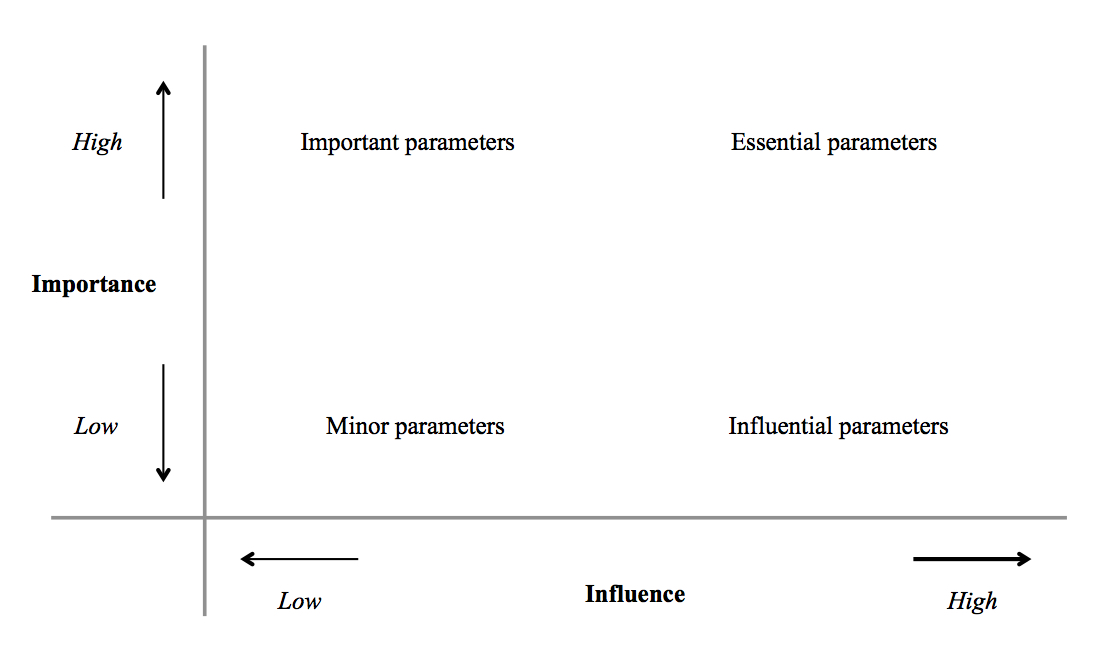
Figure 1: Parallel incorporation of local and global sensitivity analysis. Adapted from Heijungs [1996].
The importance of a parameter can originate from variability or epistemic uncertainty. A distinction between variability and uncertainty may in practice not be straightforward. However, it facilitates directions of mitigation strategies, which can be focused on essential parameters containing natural variability, and improvement of reliability, which can be focused on essential parameters that contain epistemic uncertainties (Figure 1).
Examples of parameters that are important, but not influential, are N-fertilizer rates of crop cultivation (as we showed in Groen et al. [2016]). The importance of these parameters is caused by, for example, variability in N-fertilizer rates between years. An example of parameters that are influential, but not important are parameters that can be estimated very accurately, for example, the production of N-fertilizers, and can for example be improved by innovations.
In Groen et al. [2016], we focused on developing mitigation strategies and improving reliability of results. By combining local and global sensitivity analysis the most essential input parameters for environmental impact assessment in the pork production chain can be identified. Combining the results of these two analyses allowed to derive mitigation options, either based on innovations (e.g. novel feeding strategies) or on management strategies (e.g. reducing mortality rate), and to formulate options for improving reliability of results (e.g. decreasing epistemic uncertainties). Also reliability could be improved if data quality of the most essential parameters were improved.
In Wolf and Groen et al., [2016], we focused on improving reliability of results only. By combining a local and a global sensitivity analysis, parameters could be determined which are essential to assess GHG of milk production, focusing only on the reliability of the results. Essential parameters are the emission factor of CH4 emissions from enteric fermentation, milk yield; DM feed intake of the dairy cows and the emission factor of direct N2O emission of crop cultivation. Future research can focus on reducing uncertainty and improving data quality of the most essential parameters.
A local and global sensitivity analysis should, therefore, be seen as complementary. Moreover, in most environmental impact assessment models, data availability is limited and combining local and global sensitivity analysis makes sure that parameters are not overlooked.
4. Conclusions
This thesis shows that using a systematic approach for uncertainty analysis and sensitivity analysis improves overall reliability, reduces efforts for improved data collection and supports the development of potential mitigation strategies, especially for case studies of food production, where epistemic un- certainty and variability are ubiquitous.
Methods for uncertainty analysis and sensitivity analysis can be selected depending on the available data and the research question. By combining a local and global sensitivity analysis, we can identify the most essential input parameters for environmental impact assessment. This leads to more insight in the influence and the uncertainty around the input parameters on the results, also when data availability is limited. This also allows deriving mitigation options in food production. Moreover, improving the value of uncertainty and sensitivity analysis in environmental impact assessment models, specifically in life cycle assessment and nutrient balance studies, can be increased by standardising the use of definitions and methods.
More specifically:
- Uncertainty propagation in LCA using a sampling method leads to more (directly) usable information compared to analytical uncertainty propagation [Groen et al., 2014].
- The choice for a method for global sensitivity analysis depends on the available data, the magnitude of the uncertainties in input data and aim of the study [paper under review].
- It can be predicted that including correlations among input parameters in uncertainty propagation in LCA can increase or decrease output variance. The effect of ignoring correlations on the output variance and the global sensitivity indices can be quantified, based on minimum data requirements [Groen and Heijungs, 2016] .
- Including uncertainty influences the outcome of decision-making tools. Reducing (epistemic) uncertainty of input parameters can significantly improve benchmarking of environmental performance [paper under review].
Source: General Discussion PhD thesis Evelyne Groen, An uncertain climate: the value of uncertainty and sensitivity analysis in environmental impact assessment of food, 2016
ISBN: 978-94-6257-755-8; DOI: 10.18174/375497