Evelyne Groen
Introduction: uncertainty and sensitivity analysis in environmental modeling
1. Origins of variability and uncertainty in environmental modeling
Nutrient balance analysis and life cycle assessments can both be used to develop a model that quantifies environmental impact. Collecting data for environmental impact assessment models is often perceived as a laborious task [Lloyd and Ries, 2007; Björklund, 2002]. Moreover, required data contains uncertainty due to measurement errors, or can vary widely due to natural circumstances. Most studies that quantify environmental impact, do not consider the impact of variability or uncertainties of input data on their result. Many studies aim at quantification of, for example, the carbon footprint of one kilogram of food. Most of these studies use only point values (i.e. a single value that represents a data point in the environmental impact assessment model) and overlook the range of possible realizations, and could therefore be misleading [Björklund, 2002], or might provide a false sense of accuracy [De Koning et al., 2010]. For example, nutrient balances can be used to benchmark farms, by means of quantifying the nutrient use efficiency (NUE). The NUE of one farm then is used to compare its environmental performance to other farms within the peer group. A higher NUE means that the farm is performing better. In such a situation, the peer group can learn from this farm, and incorporate similar mitigation strategies to improve their NUE. When incorporating measurements uncertainties in the calculation of the NUE, however, it might no longer be possible to rank the NUE of farms anymore, as it might not be possible to make a distinction in NUEs between the farms.
Origins of variability and uncertainty in environmental impact assessment models can be divided into two broad categories: (I) natural variability and (II) epistemic uncertainty.
- Natural variability relates to observable variation, which means it is inherent to the system and therefore cannot be reduced [Walker et al., 2003]. Although it is possible to strive for reduction of natural variability in time or space, the observed variation cannot be reduced. An example of natural variability in agriculture is variation between annual crop yields of wheat, which exist in time, i.e. across years, and in space, i.e. across countries or soil types. Another example is the variation in diet preferences amongst consumers, which makes it impossible to calculate the carbon footprint of one day of food.
- Epistemic uncertainty originates from a lack of knowledge and can be reduced by gaining more or better data [Walker et al., 2003]. Epistemic un certainty includes errors from measurement instruments, or those introduced by the observer. For example, in case a weighting scale is not available to determine the weight of a cow, the weight can be estimated based on body measurements, such as body length, heart girth and height [Francis et al., 2004; Lesosky et al., 2012]. Literature shows that body weight can be esti- mated from single heart girth measurements with reasonable accuracy. Heart girth measurements, however, can result in measurement errors because the positioning of the cow can easily affect the result [Heinrichs et al., 1992].
More sources of natural variability and epistemic uncertainty are found in Table 1.
Table 1: Examples of natural variability and epistemic uncertainty.
| Category | Examples of sources |
|---|---|
| Natural variablity | Climate variability, soil type, genetic differences, variation in temperature, differences in management strategies, geographical differences, consumer preferences |
| Epistemic uncertainty | Measurement errors, errors in observations, errors of measurement instruments, estimates of experts, lack of knowledge |
However, the theoretical distinction made between natural variability and epistemic uncertainty, may be not so clear in practice. An example is the epistemic uncertainty ranges that are given by the intergovernmental panel on climate change (IPCC) around the emission factors of N2O from application of fertilizer. This range is often interpreted as epistemic uncertainty, but might include also natural variation due to differences in climate conditions or soil types, which is in fact caused by natural variability. Both natural variability and epistemic uncertainty are also found for the parameter annual milk yield per cow. Annual milk yield per cow can vary naturally due to genetic differences, or differences in feeding strategies, whereas milk yields can also be prone to the same measurement error (i.e. epistemic uncertainty).
Many experience natural variability or epistemic uncertainty around data for input parameters in environmental assessment models, making the exact environmental impact difficult to quantify.
2. Incorporating variability and uncertainty in environmental impact assessment
Uncertainty analysis can be used to propagate epistemic uncertainties and natural variability of input parameters through an environmental impact assessment model (Box 1). From now on, when the term uncertainty analysis is used, it can refer to the analysis of the magnitude and consequences of both epistemic uncertainty and natural variability of the input parameters. The term uncertainty in uncertainty analysis can be interpreted as a quantitative value either representing epistemic uncertainty or natural variability (in this thesis). An uncertainty analysis quantifies the uncertainty of the output based on the uncertainty of the input parameters. For example, what is the uncertainty around greenhouse gas emissions of 1 kg of milk? These types of methods require the knowledge of a distribution function (e.g. a normal distribution), or a least a parameter of dispersion, such as the variance, to propagate the input uncertainties through the environmental impact assessment model.
In addition to the uncertainty analysis, a sensitivity analysis can be used to study the effect of input uncertainties on the output of an environmental impact assessment model. Two commonly used approaches for sensitivity analysis are local sensitivity analysis and global sensitivity analysis. Terminology often used in case of uncertainty analysis and sensitivity analysis is defined in Box 1.
Box 1: Definitions of uncertainty (analysis) and sensitivity (analysis).
| Uncertainty versus sensitivity |
|---|
| Uncertainty: a property attributable to an input parameter or an output parameter. In the context of this thesis it relates to quantitative uncertainty. Uncertainty of the input parameters can be given as a probability distribution function (for instance, a normal distribution with a specified mean and standard deviation). Uncertainty analysis refers to the estimation of the uncertainty attribute of a model output using the uncertainty attributes of the model inputs. |
| Sensitivity: a property attributable to how a model output behaves as the result of the variation of an input parameter [Saltelli et al., 2008]. There are three types of sensitivity analyses: (1) a local sensitivity analysis addresses what happens to the output when input parameters are changed, i.e. the intrinsic model behavior of a parameter. The parameters that have the largest effect on the model output are referred to as the most influential parameters; (2) a screening analysis addresses what happens to the output based on the uncertainty range of the different input parameters; and (3) a global sensitivity analysis addresses how much the uncertainty around each input parameter contributes to the output variance [Saltelli et al., 2008]. Both the screening analysis and the global sensitivity analysis combine the intrinsic model behavior with the information of uncertainty around input parameters. The parameters that change the model output most or explain most of the output variance are referred to as the most important parameters. |
Most studies of environmental impact assessment models assume that the input parameters can vary independently [Lloyd and Ries, 2007; Bojacá and Schrevens, 2010]. However, in certain cases correlations exist between input parameters, for example, a correlation can be expected between crop yield and fertilizer. This means that if fertilizer rate is increased, crop yield (to some extent) also increases. Including correlations in the sampling design can answer questions such as: what is the effect of including correlations between crop yield and fertilizer on the model output? What is the effect of including correlations between input parameters on the global sensitivity analysis? Including correlations can affect both uncertainty analysis and sensitivity analysis, but requires information of the presences of correlations coefficients of the input parameters, such as the variance for uncorrelated parameters or a covariance for correlated parameters, to propagate the input uncertainties through the environmental impact assessment model.
A local sensitivity analysis quantifies the effect on the output when an input parameter is changed. For example, what would be the effect on greenhouse gas emissions per kg of milk when a cow would produce 5% more milk with the same amount of feed? In general, these type of methods consider the effect of a change independent of other input parameters and do not consider the actual range over which the input parameters can vary (Figure 1). These types of methods are especially useful when data availability is limited to point values.
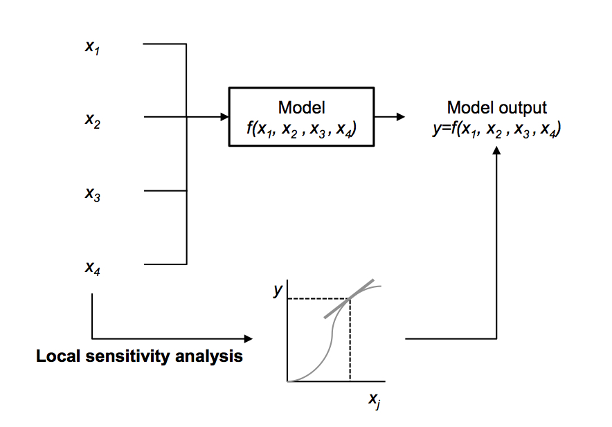
Figure 1: An illustration of a local sensitivity analysis for a model with four input parameters (x1, ... , x4). Each input parameter is changed independently; the influence of parameter x1for example, can be expressed as the effect of changing x1 on the output y. Source: General Introduction PhD thesis Evelyne Groen "An uncertain climate: the value of uncertainty and sensitivity analysis in environmental impact assessment of food", 2016.
A screening analysis quantifies the effect on the output when an input parameter is changed according the to uncertainty range of an input parameter. For example, what would be the effect on greenhouse gas emissions per kg of pork when variation of manure production in pigs vary with 3%? In general, this type of method also considers the effect of a change independent from other input parameters. These types of methods are especially useful when only little information is available on the input uncertainties.
A global sensitivity analysis can be seen as an extension of uncertainty propagation: it determines how much each input parameter contributes to the output variance. A global sensitivity analysis considers the actual variation over all input parameters simultaneously (Figure 2). For example, how much does the annual variation around crop yield of wheat contribute to the uncertainty around the greenhouse gas emissions? What is the impact of incorporation of covariance on the global sensitivity analysis? In general (but not always), these methods require full knowledge of the input uncertainties (i.e. distribution functions) and information regarding the covariance if the input parameters are correlated.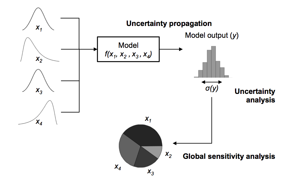
Figure 2: An illustration of a global sensitivity analysis for a model with four parameters: the variance decomposition (pie chart) explains the output variance (histogram), given the distribution functions of the four input parameters on the left hand side of the figure. Source: General Introduction PhD thesis Evelyne Groen "An uncertain climate: the value of uncertainty and sensitivity analysis in environmental impact assessment of food", 2016.
Incorporating uncertainty in an environmental impact assessment model will strengthen the model outcomes. It will provide knowledge about the range of model outputs, which enables more informed decision-making. At present, however, a standardized methodology how to propagate uncertainties or which type of sensitivity analysis to use, is missing.
Knowledge gaps
To determine the effect of input uncertainties on the output, most environmental impact assessment studies that performed a local sensitivity analysis use a straightforward method, i.e. a one-at-a-time (OAT) approach. An OAT approach varies an input parameter with, e.g. 5 or 10%, and subsequently quantifies the impact on the model output [Suh and Yee, 2011; Van Middelaar et al., 2012; Van Zanten et al., 2015; Yang et al., 2011]. This procedure is usually repeated for a limited number of input parameters. The input parameters that cause most change in model output are considered to be the most influential parameters. The OAT approach, however, has two weaknesses:
- the number of input parameters assessed is usually a subset of the total available input parameters, implying that potential influential parameters might be overlooked;
- the actual uncertainty ranges of input parameters are ignored: some input parameters may vary only with 5%, while others may vary with a factor ten or hundred. Their impact on the model output, therefore, might be under- or overestimated.
The following methods are ordered on increased knowledge around the uncertainties of the input parameters:
- Point values Even if no other data are available than the point values used in the model, a local sensitivity analysis can be performed. The multiplier method Heijungs and Suh [2002]; Heijungs, 2010] (MPM), for example, determines the local sensitivity of all input parameters in an LCA model, and does not require actual ranges over which input parameters can vary. The MPM, therefore, accommodates the first weakness of OAT methods mentioned, as it systematically explores the sensitivity of all input parameters. MPM can be used to explore areas of potential mitigation options [Heijungs, 1996]. Once these parameters are indicated, a further examination is required to see if these parameters can be improved, by e.g. technical innovations or by improving management. However, since MPM only quantifies the intrinsic sensitivity of the input parameters within the model, and does not include the actual uncertainty of the input parameters, this method is less suitable to make comparisons between products on their environmental performance.
- Ranges In case only limited amount of data is available, for example, the ranges of input parameters are known, a screening analysis can be performed. The method of elementary effects [Saltelli et al., 2008 ; Campolongo et al., 2007] (MEE), for example, calculates the sensitivity of input parameters based on their actual ranges, by exploring model outputs of those ranges. MEE can be used to determine how uncertainty around the input parameters affects the output. MEE does include an uncertainty range for each input parameter, and, therefore, partly accommodates the second weakness of the OAT approach. Also, this screening analysis can be used to indicate important parameters that contain opportunities for improvement regarding environmental performance [Saltelli et al., 2008 ; Campolongo et al., 2007]. Since MEE is a screening analysis, it is can also be used to find parameters that should be taken into account in a subsequent global sensitivity analysis, i.e. it focuses the data collection to the most important parameters before performing a global sensitivity analysis. As only the ranges are used of the input parameters, because the distribution functions could not (yet) be defined, the uncertainty of the model output is of limited value. For example, the model output of the MEE method cannot be used to determine significant differences between two product alternatives, which can be done with uncertainty propagation of distributions functions using Monte Carlo simulation.
So far, no study combined the MPM and MEE in an environmental impact assessment model, to see if a combination of methods leads to more insight in parameters that can contain potential improvement options, or if their uncertainty needs to be reduced to improve the reliability of the results.
-
Distribution functions (I) In case full knowledge about the uncertainties is available, including the distribution function (e.g. a normal distribution), mean and a parameter of dispersion (e.g. standard deviation), uncertainty propagation and uncertainty analysis can be performed by means of e.g. a simulation based on stochastic sampling.
Current practice in LCA is dominated by one type of sampling, namely Monte Carlo sampling [Lloyd and Ries, 2007], but there are several other methods to propagate uncertainties [Lloyd and Ries, 2007], such as Latin hypercube sampling, which uses a smart sampling design that can potentially reduce the sample size of the simulation, just as (randomized) quasi Monte Carlo sampling. Fuzzy interval arithmetic [Lloyd and Ries, 2007], makes use of only three data points (mean, minimum and maximum value) to propagate uncertainties, analytical uncertainty propagation [Heijungs, 1996], uses only the mean and a parameter of dispersion to propagate uncertainties. However, these methods have not been compared in a consistent manner to see if one of these methods performs better than the other.
- Distribution functions (II) After uncertainty propagation, a global sensitivity analysiscan be performed that can be used to explain where the output uncertainty comes from, i.e. which parameters are most important in explaining the output variance. A global sensitivity analysis can also be used to determine which of the input parameters contribute only minor to the output variance and thus can be set to a fixed value to simplify data collection of similar future studies [Saltelli et al., 2008].
In LCA literature, different methods for global sensitivity analysis have been used that quantify the contribution to output variance. Sampling-based methods employ regression-like techniques that use the distribution function, such as the squared standardized regression coefficients and the squared Pearson correlation coefficient or squared Spearman (rank) correlation coefficient [Saltelli et al., 2008]. In contrast, analytical methods (the so-called key issue analysis; [Heijungs, 1996]) only require a parameter of dispersion to calculate the contribution to the output variance for each parameter. Outside the LCA domain, a much wider set of methods have been developed and applied, such as random balance design and the Sobol’ method [Sobol’, 2001; Saltelli et al., 2008], which also both use the distribution functions. So far, the application of different methods for global sensitivity analyses in environmental impact assessment models, such as LCAs and nutrient balances, have been limited. For these methods, it is not known if there is one method that performs better than the other methods.
A common strategy in environmental impact assessment models, is to look for improvement options, and to do so, two product alternatives are compared. A suitable approach is to use a discernibility analysis [Henriksson et al., 2015; Heijungs and Kleijn, 2001], where random drawings from two sampling (e.g. Monte Carlo) runs are compared and a frequency distribution is determined of how much one alternative is better than the other. Incorporating uncertainties in this way, improves environmentally friendly decision-making and benchmarking.
So far, no study has yet combined the knowledge of a global sensitivity analysis in a benchmarking study in environmental impact assessment models, such as a nutrient balance, to see if reducing input uncertainties influence the result of benchmarking.
In addition, very few studies incorporated correlations in the sample design of environmental impact assessment models [Wei et al., 2014; Bojacá and Schrevens, 2010]. So far, no study has yet included the effect of correlations on the global sensitivity analysis in environmental impact assessment model and applied it to a case study of food production. Moreover, none explored how to quantify the effect of ignoring correlations between input parameters on the output variance and in global sensitivity analysis.
Even though case studies of food production are especially prone to natural variability and epistemic uncertainties, very few case studies made a thorough examination of all the parameters in the model.
Source:Intoruduction PhD thesis Evelyne Groen, An uncertain climate: the value of uncertainty and sensitivity analysis in environmental impact assessment of food, 2016
ISBN: 978-94-6257-755-8; DOI: 10.18174/375497